Test Waveprop class

Define a BarSingle bar and use it with Waveprop to compute elastic wave propagation in simple test cases.

# sphinx_gallery_thumbnail_number = 5

import matplotlib.pyplot as plt
import numpy as np

from elwaspatid import Waveprop, BarSingle, trapezeWave

Define material and geometrical parameters

E = 201e9  # Young modulus [Pa]
rho = 7800  # Density [kg/m3]
d = 0.020  # diameter [m]
k = 2.4  # diamters ratio [-]

Define the incident wave vector

incw = np.zeros(80)  # incident wave
incw[0:20] = 1e3  # >0 means traction pulse

Create the bars

dx = 0.01  # length of an elementary Segment [m]
n = 50  # number of Segments [-]
D = np.ones(n) * d  # diameters of the Segments
bb = BarSingle(dx, D, E, rho)  # constant section bar
D2 = np.hstack((np.ones(n)*d, np.ones(n)*d*k))  # section change
b2 = BarSingle(dx, D2, E, rho)  # cross-section increase
b3 = BarSingle(dx, D2[::-1], E, rho)  # cross-section reduction

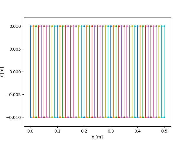
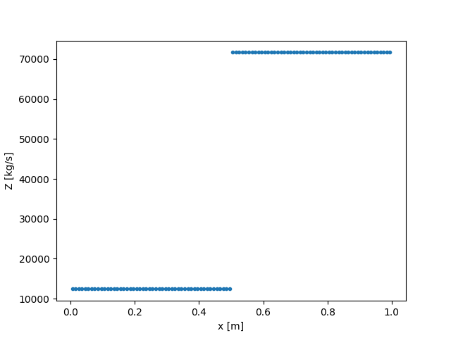
# Visualize the bar:
bb.plot()  # constant cross-section and constant impedance
b2.plot()  # cross-section and impedance increase

• 
• 
• 
• 

Free-free uniform bar

Incident pulse reflects on both end of the bar endlessly. The force at both ends of the bar is null. Traction reflects as compression. Compression pulse reflects as traction.

test = Waveprop(bb, incw, nstep=2*len(incw), left='free', right='free')
test.plot()

• 
• 

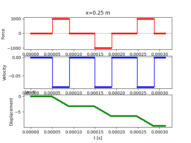
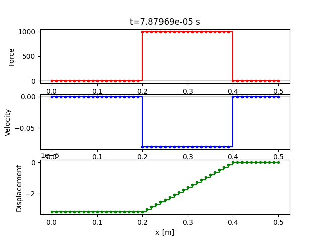
It is possible to plot cuts of the space-time diagram, at a given time t or at a given position x

test.plotcut(x=bb.x[int(n/2)])
test.plotcut(t=bb.dt*len(incw)/2)

• 
• 

Additional diagrams are also available

test.plot(typ='dir-D')  # Wave direction (dir) and Displacement (D)
test.plot(typ='sig-eps')  # Stress (sig) and Strain (eps)

• 
• 
• 
• 

Free-fixed uniform bar

Left end is free, right end is fixed:

• compression relfects as compression on fixed end;

• then, compression reflects as traction on free end;

• and finally traction reflects as traction on fixed end.

Note that velocity and displacement of the right end are null.

test = Waveprop(bb, incw, nstep=3*len(incw), left='free', right='fixed')
test.plot()
test.plot(typ='D')  #  Displacement (D)

• 
• 
• 

Infinite-infinite uniform bar

Infinite end amounts to anechoic condition: no reflecion of elastic wave.

testf = Waveprop(bb, incw, nstep=100, left='infinite', right='infinite')
testf.plot()

• 
• 

Free-free bar with section increase

The traction pulse reflects as traction on section increase.

testa = Waveprop(b2, incw, nstep=170, left='free', right='free')
testa.plot()

• 
• 

Free-free bar with section reduction

The traction pulse reflects as compression on the section reduction.

testd = Waveprop(b3, incw, nstep=170, left='free', right='free')
testd.plot()

• 
• 

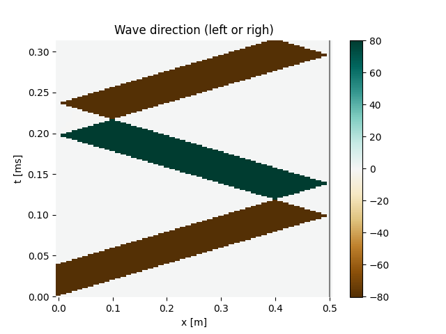
Whatever pulse input is possible

Trapeze

For exemple, define a trapeze pulse shape and propagate it in a bar with constant section. Right end is free so the traction wave is reflected as a compression wave. Left end is infinite so no reflecion occur.

trap = trapezeWave(plateau=5, rise=5)
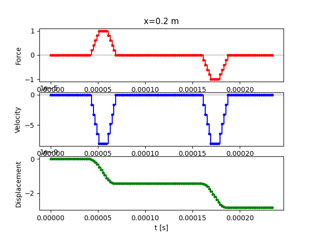
testt = Waveprop(bb, trap, nstep=120, left='infinite', right='free')
testt.plot()
testt.plotcut(x=0.2)

• 
• 
• 

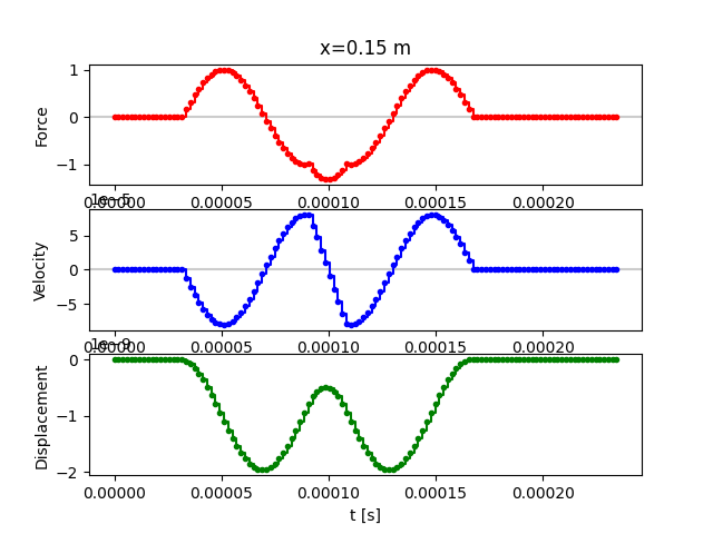
And why not a sine pulse?

sine = np.sin(2*np.pi*np.linspace(0, 1, num=40))
bar = BarSingle(dx, np.ones(30)*d, E, rho)
tests = Waveprop(bar, sine, nstep=3*len(sine), left='infinite', right='free')
tests.plot()
tests.plotcut(x=0.15)
tests.plotcut(x=0.20)

plt.show()

• 
• 
• 
•